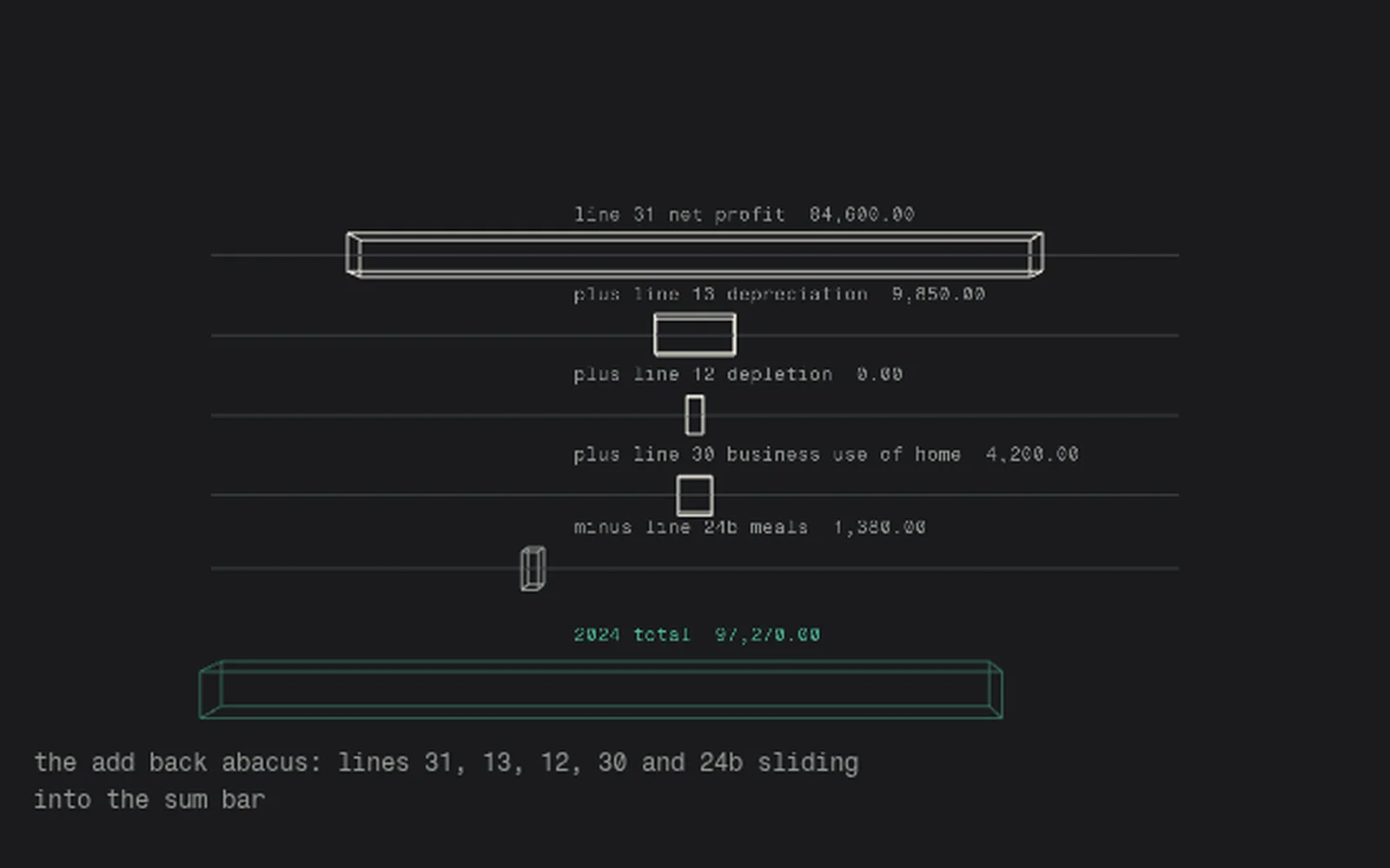

Take the 2024 return out of the file and turn to Schedule C. Line 31 says net profit, and on the sample file this note follows all the way through (Sample Mortgage Co., LN 2026090412, borrower R.M., underwriter of record J. Ortiz, DE) it reads $84,600.00. That is where the worksheet starts. It is not where it ends, and the distance between the two is the whole point of Form 1084.
What line 31 leaves out
Net profit is what was left after every expense the return allowed, and some of those expenses never left the borrower's account as cash. Depreciation is the obvious one. A truck bought in 2023 keeps reducing profit on paper for years while the money went out once. Fannie Mae's Form 1084, the Cash Flow Analysis, exists to put that cash back where the borrower can spend it, one line at a time, with a page behind each line. Freddie Mac's Form 91 does the same job from the same Schedule C lines, so everything below reads across to a Freddie Mac file without changing a number.
The four lines that come back, and the one that goes out
Line 13, depreciation. Added back in full. It is a non cash expense and the largest add back on most Schedule C files. On the sample file it is $9,850.00 for 2024, on page 47 of the upload.
Line 12, depletion. Added back for the same reason. Most service businesses show zero here and the sample file does too. The row still prints, with its zero, because a blank cell is where a QC reviewer's question starts.
Line 30, business use of home. Added back. The borrower's housing cost already sits on the liability side of the application, so leaving it inside the business expenses would count it twice. $4,200.00 on the sample file, page 47.
Line 24b, meals. This one goes the other way. The return allowed only part of what the borrower spent on meals as an expense; the rest still left the business account, so the worksheet subtracts line 24b rather than pretending the cash stayed. $1,380.00 for 2024.
Amortization and casualty losses have their own rows on the form and follow the depreciation logic. The sample file has neither, so those rows print zero and stay on the sheet.
2024 on the page
Net profit 84,600.00, plus depreciation 9,850.00, plus depletion 0.00, plus business use of home 4,200.00, minus meals 1,380.00. Total for 2024: 97,270.00.
Every one of those figures carries the cite p.47, because page 47 of the upload is where the 2024 Schedule C sits. The cite is printed beside the figure, in the same row, not in a footnote at the bottom of the sheet. An underwriter checking one number should not have to hunt for the page.
2025 on the page
Now the 2025 return, which is page 52. Net profit 92,150.00. Depreciation 10,400.00, a second vehicle having gone into service. Depletion 0.00. Business use of home 4,200.00 again. Meals 2,120.00, subtracted. Total for 2025: 104,630.00.
Two years, two totals, two pages.
| line | 2024 p.47 | 2025 p.52 |
|---|---|---|
| net profit, line 31 | 84,600.00 | 92,150.00 |
| plus depreciation, line 13 | 9,850.00 | 10,400.00 |
| plus depletion, line 12 | 0.00 | 0.00 |
| plus business use of home, line 30 | 4,200.00 | 4,200.00 |
| minus meals, line 24b | 1,380.00 | 2,120.00 |
| total | 97,270.00 | 104,630.00 |
Why 24 and not 12
The rule for a self employed borrower with two full years of returns is the average, and the worksheet writes the average as a 24 month figure: 97,270.00 plus 104,630.00 is 201,900.00, and 201,900.00 divided by 24 is $8,412.50 a month. The result is the same as averaging two annual figures and dividing by twelve. Writing it in months is a habit worth keeping, because when a year to date profit and loss statement is added later the months on the sheet stay honest instead of turning into a fraction of a year nobody wrote down.
Before the average is used, the trend is checked. 2025 is up 7.6 percent on 2024, which is stable and rising, so the two year average is the qualifying figure. Had 2025 come in lower than 2024, the average would not be used at all; the rule takes the more recent, lower year and asks for a reason the decline will not continue. The worksheet prints the trend either way, so the reader sees which rule applied and why without redoing the division.
What the AUS had
The loan officer entered $7,568.75 in the AUS. That figure is not so much wrong as incomplete: it is the same two year average with everything in it except depreciation. 20,250.00 of depreciation across the two years, divided by 24, is 843.75, and $7,568.75 plus $843.75 is $8,412.50 to the cent. The worksheet prints both figures side by side with the difference and the line that caused it, because the DU or LPA findings were run on the lower figure and the underwriter will want to decide whether to run them again.
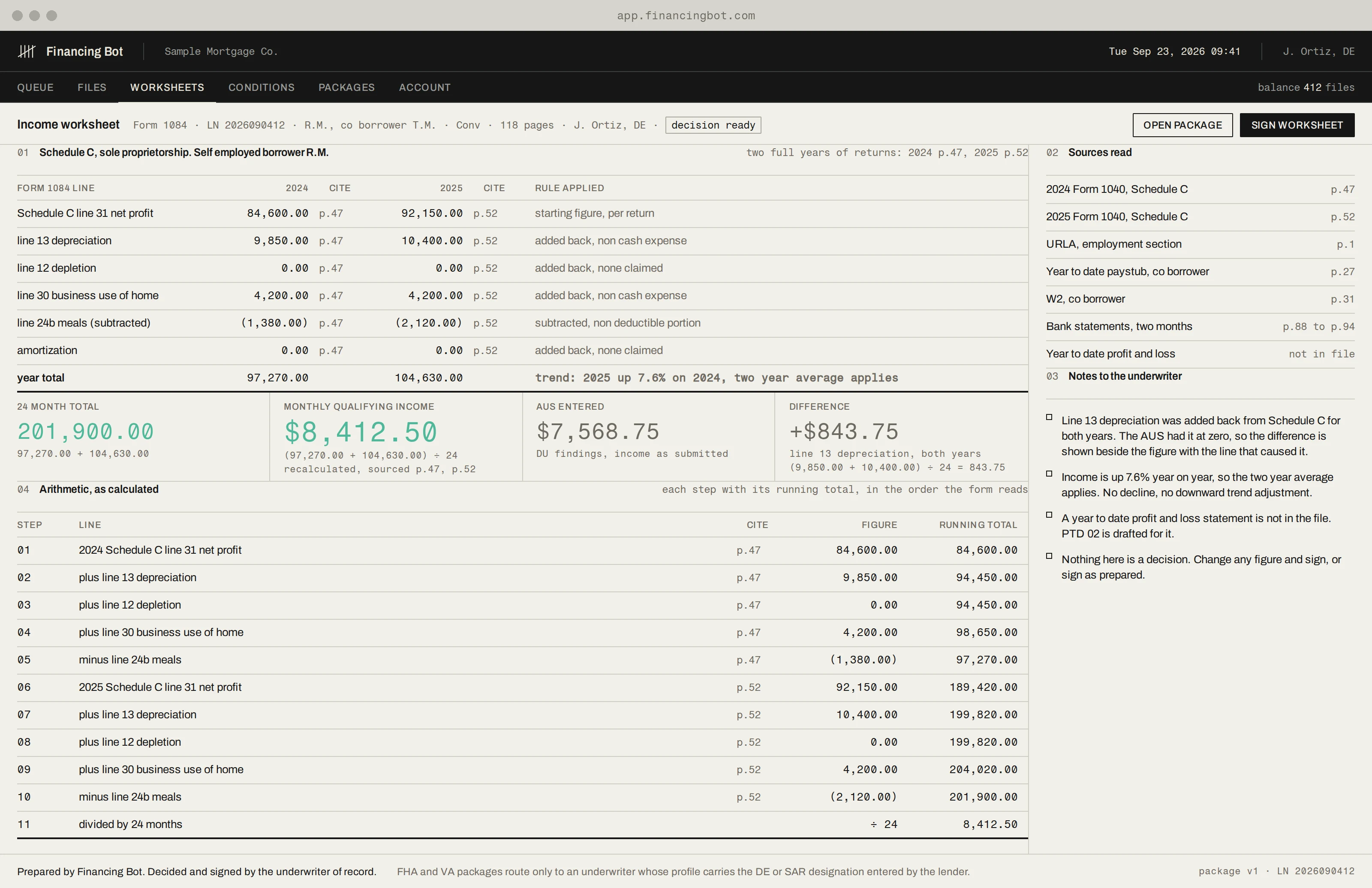
Nothing on that sheet is a recommendation; it is arithmetic with an address.
What goes in the package
The worksheet, the two Schedule C pages it cites, the trend line, and the AUS comparison. The figure that was recalculated and sourced is the only one printed in the accent color, so it can be found in a second on a busy sheet. Nothing on that sheet is a recommendation; it is arithmetic with an address. The underwriter reads it, changes any line they disagree with (the original stays beside the edit), and signs.
If you'd rather see this run on your own Schedule C files than on a sample, that is what a file pack is for.